
SKEW-T BASICS
The Skew-T Log-P offers an almost instantaneous snapshot of the atmosphere from the surface to about the 100 millibar level. The advantages and disadvantages of the Skew-T are given below:
Why do we need Skew-T Log-P diagrams?
- Can assess the (in)stability of the atmosphere
- Can see weather elements at every layer in the atmosphere
- Determine cap strength, convective temperature, forecasting temperatures,
determine character of severe weather - This is the data used to produce the synoptic scale forecast models
What are some disadvantages of Skew-T’s?
- Only available twice a day (00Z and 12Z)
- Character of weather can change dramatically between soundings
- Sounding does not give a true vertical dimension since wind blows balloon downstream
- Sounding does not give true instantaneous measurements since it takes several minutes to travel from the surface to the upper troposphere
Below are all the basics lines that make up the Skew-T
Isobars— Lines of equal pressure. They run horizontally from left to right and are labeled on the left side of the diagram. Pressure is given in increments of 100 mb and ranges from 1050 to 100 mb. Notice the spacing between isobars increases in the vertical (thus the name Log P).
Isotherms– Lines of equal temperature. They run from the southwest to the northeast (thus the name skew) across the diagram and are SOLID. Increment are given for every 10 degrees in units of Celsius. They are labeled at the bottom of the diagram.
Saturation mixing ratio lines– Lines of equal mixing ratio (mass of water vapor divided by mass of dry air — grams per kilogram) These lines run from the southwest to the northeast and are DASHED. They are labeled on the bottom of the diagram.
Wind barbs– Wind speed and direction given for each plotted barb. Plotted on the right of the diagram.
Dry adiabatic lapse rate– Rate of cooling (10 degrees Celsius per kilometer) of a rising unsaturated parcel of air. These lines slope from the southeast to the northwest and are SOLID. Lines gradually arc to the North with height.
Moist adiabatic lapse rate— Rate of cooling (depends on moisture content of air) of a rising saturated parcel of air. These lines slope from the south toward the northwest. The MALR increases with height since cold air has less moisture content than warm air.
Environmental sounding— Same as the actual measured temperatures in the atmosphere. This is the jagged line running south to north on the diagram. This line is always to the right of the dewpoint plot.
Dewpoint plot– This is the jagged line running south to north. It is the vertical plot of dewpointtemperature. This line is always to the left of the environmental sounding.
Parcel lapse rate— The temperature path a parcel would take if raised from the Planetary Boundary Layer. The lapse rate follows the DALR until saturation, then follows the MALR. This line is used to calculate the LI, CAPE, CINH, and other thermodynamic indices.
Below is an example diagram showing the lines of the Skew-T Log-P diagram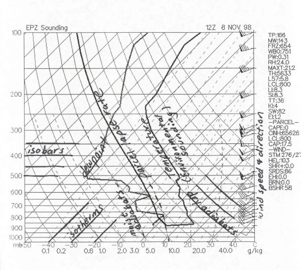
| INTERPRETATION OF SKEW-T INDICES |
To the right of most Skew-T diagrams on the web there will be a list a parameters and indices. To a first timer, these letters and numbers look as a collection of abbreviations and random numbers. With experience in examining Skew-T data on a daily basis, you will be able to instantly interpret the abbreviations and numbers. The numbers will also have meaning since they can be classified into categories.
This section interprets most of those values and gives operational significance to the values. Each parameter or indice will be broken down one by one. In a severe weather situations and during inclement weather, these indices come in handy. The indices should be used as guides. Often, indices will contradict each other and can change rapidly in the course of a couple of hours. An experienced meteorologist is well informed to how a sounding will change throughout the day and why some sounding indices are better than others in certain situations. Soundings are most notably changed through thermal advection, moisture advection, and evaporative cooling. Modified soundings should be studied along with the standard 12 Z and 00Z sounding.
Interpretation of Skew- T Log-P Indices
WMO: 4-letter station identification number
TP: Tropopause Level
- Location in millibars of the tropopause, generally near 150 millibars
FRZ: Pressure level at which the environmental sounding is exactly zero degrees Celsius
- Find intersection of 0-degree isotherm with environmental sounding
WBO: Wet bulb zero temperature. Value at which the sounding is at zero degrees Celsius due to evaporative cooling. Value is given as a pressure level. This value will always be at a higher pressure (closer to the surface) than the FRZ level unless the sounding is saturated.
- Value found through computer algorithms (once the wet bulb is found for every pressure level, the wet bulb zero can then be located.)
- Wet bulb temperature can be found by the following sequence.
1. Pick a pressure level
2. Find LCL from that pressure level
3. From LCL go back down the sounding at the wet adiabatic lapse rate to the original pressure4. This temperature is the wet bulb temperaturePW: Value of precipitable water in inches
- This is the amount of liquid water on the surface after all water in all three phases is brought to the surface
- Greater than 1.75 inches represents a water loaded sounding
- less than 0.75 inches represents a fairly dry sounding
RH: The average relative humidity between the surface and 500 millibars.
- 0 to 40% very low
- 41 to 60% low
- 61 to 80% moderate
- 81 to 100% Moist
Relative humidity is a good measure of the evaporational drying power of the air and how close the atmosphere is to saturation. It does not, however, tell you how much moisture mass there is in the air.
MAXT: Estimated maximum afternoon temperature. Most relevant when using a morning sounding. Most accurate on days with clear skies and moderate winds.
L57: 700 to 500 millibar lapse rate
- Less than 5.5 stable
- 5.5 to 9 conditionally unstable (unstable if moist in PBL)
- 9 or greater Incredibly unstable
- Atmosphere is stable when the environmental lapse rate is less than the moist adiabatic lapse rate. Especially true iflarge inversion is present.
- Atmosphere is conditional unstable when the environmental lapse rate is between the moist and dry adiabatic lapse rate
- Atmosphere is absolutely unstable if environmental lapse rate is greater than the dry adiabatic lapse rate
LCL: Lifted condensation level in millibars using surface data. This is the level in the atmosphere clouds will form if forced lifting takes place. LCL is found by the following process
- draw a dry adiabat from the surface temperature
- draw a mixing ratio line from the dewpoint
- intersection is the LCL
LI: Lifted Index. This is the temperature difference between the environmental and parcel temperatures at the 500 mb level.
- 500 mb envir. Temp – 500 mb parcel Temp = LI
- 0 or greater= stable
- -1 to -4= marginal instability
- -5 to -7= large instability
- -8 to -10= extreme instability
- -11 or less = ridiculous instability
SI: Showalter index. Same as LI, except parcel is lifted from 850 mb. Use SI instead of LI in the cool season especially when surface is capped by a cool front.
TT: Total totals index. (T850 – T500) + (Td850 – T500)
Vertical totals + cross totals - <44 convection not likely
- 44 to 50 convection likely
- 51- 52 isolated severe storms
- 53- 56 widely scattered severe storms
- Greater than 56 scattered severe storms
Limitations: large lapse rates can produce large TT values with little low level moisture
TT is region specificKI: K index. (T850 – T500) + (Td850 – Tdd700)
Lapse rate + available moisture - less than 15 Convection not likely
- 15 to 25 Small potential for convection
- 26 to 39 Moderate potential for convection
- 40+ High potential for convection
Limitations: Favors non severe convection. This index is a measure of thunderstorm potential but has nothing to do with severity of storms. Can not be used in mountain areas
SW: Sweat Index. Severe WEAther Threat index . Indice combining many thermodynamic and wind values.
SWEAT= 12(850Td)+20(TT-49)+2(V850)+(V500)+125(sin(dd500-dd850)+.2) If TT less than 49, then that term of equation is set to zero - 150 to 300 Slight severe
- 300 to 400 Severe storms possible
- 400+ Tornadic severe storms possible
Formula covers: low level moisture, instability, low level jet, upper level jet, warm air advection
EI: Energy Index
CAPE: Convective Available Potential Energy. This is the positive area on a sounding (the area between the parcel and environmental temperature)
- 1 to 1,500 Positive CAPE
- 1,500 to 2,500 Large CAPE
- 2,500 + Extreme CAPE
Max upward vertical velocity = (2*CAPE)^1/2, does not take into consideration water loading, entrainment
CINH: Convective Inhibition. This is the negative area on a sounding. A large cap or a dry planetary boundary layer will lead to high values of CINH and stability
CAP: Cap strength in degrees Celsius. Values above 2 indicate convection will not occur within at least the next couple of hours. Cap needs to be less than 2 in general before it can be broken.
EL: Equilibrium level. The pressure value at the top of the positive CAPE area
MPL: Maximum parcel level. Highest level a parcel can rise in the atmosphere. This value is above the EL due to the updrafts momentum.
STM: Estimated storm motion. Storm will be moving from X and X knots.
HEL: Helicity Amount of streamwise vorticity available for ingestion into a storm. Streamwise vorticity is a function of low level inflow and horizontal vorticity generated by speed shear with height or directional shear with height in the PBL.
- 150 to 300= possible supercell
- 300 to 400= supercell severe storms
- 400+ = Tornadic supercells possible
SHR: Positive shear in the 0 to 3000m above ground level. Units are in time to the negative 1. Dividing the change in vertical wind speed by the change in the distance derives these units. Km/hr divided by km = hr-1. Value is found by finding the change in wind speed from the surface to 3000m and dividing that value by 3000m (3 km).
- 0 to 3 weak
- 4 to 5 moderate
- 6 to 8 large
- 9+ very large
SRDS: Storm relative directional shear
EHI: Energy helicity index. = (SR HEL * CAPE) / 160,000
- EHI > 1 Supercells likely
- EHI from 1 to 5 F2, F3 tornadoes possible
- EHI 5+ F4, F5 tornadoes possible
BRN: Bulk Richardson Number = (CAPE / 0-6km shear)
- less than 45 Supercells
- less than 10 Environment too sheared
- Teens Optimum for severe storms, good balance of CAPE and shear
BSHR: Bulk shear value (magnitude of shear over layer)
CCL: Level at which condensation will occur if sufficient afternoon heating causes rising parcels of air to reach saturation. The CCL is greater than or equal in height (lower or equal pressure level) than the LCL. The CCL and the LCL are equal when the atmosphere is saturated.
- found at the intersection of the saturation mixing ratio line (through the surface dewpoint) and the environmental temperature.
Level of Free Convection (LFC)– The level at the bottom of the area of positive CAPE. If a parcel reaches this level it will begin to accelerate in the vertical.
Relative Humidity– Found by dividing the mixing ratio by the saturation mixing ratio or the vapor pressure divided by the saturation vapor pressure.
- Find the saturation mixing ratio value that runs through the dewpoint and the temperature. Next, divide the dewpoint mixing ratio by the temperature mixing ratio.
Potential Temperature– Temperature found by lifting or descending a parcel to the 1000 mb level from the pressure level of interest.
Equivalent Potential Temperature– Also known as THETA-E. Temperature of a parcel after all latent heat energy is released in a parcel then brought to the 1000 mb level.
Wet Bulb potential temperature– Found the same as the wet bulb. When the wet bulb value is found, keep descending wet adiabatically to the 1000 mb level.
Convective instability– Occurs when a dry layer overlays a warm and humid layer. Lifting of atmosphere causes the lapse rate to increase since the lower layer cool at the WALR while the dry layer cools at the DALR.
Hydrolapse– Rapid increase or decrease in dewpoint with heightFrom pressure of interest (typically the surface) find the LCL, lift the parcel wet adiabatically to 100 mb. Next, descend the parcel dry adiabatically to the 1000 mb level. The temperature at 1000 mb of this parcel is the THETA-E.
| THERMODYNAMIC IMAGES |
There are 4 charts which will be discussed in this section which are extremely important to severe weather forecasting. The charts include: CAPE, Helicity, Energy Helicity Index, and the 850-500 relative humidity/ Lifted Index plot. An example of each chart is shown along with operational interpretation. One location these plots are available are on UNISYS weather at:
http://weather.unisys.com/nam/index.php
CLICK THE TITLE TO SEE THE CURRENT ONLINE IMAGE FOR EACH
Online images: CAPE
*Largest CAPE will occur in the warm sector of a mid-latitude cyclone
*Interpretation of values:
*1 to 1,500 Positive CAPE
*1,500 to 2,500 Large
*2,500+ Extreme
*High values of CAPE will result in high values of upward vertical velocity in the updraft region of a thunderstorm
*CAPE is increased by low level warm air advection, daytime heating, low level moisture advection (high low level dewpoint), upper level cold air advection (cooling temperature in mid-levels)
*CAPE values tend to be highest in the warm season (especially late Spring)
Online images: HELICITY
*Low level inflow, speed shear and directional shear maximize helicity values
*Helicity values tend to be highest ahead of cold fronts and near warm fronts within the warm sector of a mid-latitude cyclone
*Interpretation of values:
*150-300 Possible Supercell
*300 to 400 Supercell Severe Favorable
*400+ Tornadic Thunderstorms Favorable
*The Low Level Jet can amplify low level inflow. Higher winds lead to a more rapid rotation of air if shear exists
*Differential advection and surface friction cause speed and directional shear
*Helicity is the amount of streamwise vorticity available for ingestion into thunderstorms. Streamwise vorticity is the amount of parallel inflow to horizontal vorticity
Online images: ENERGY HELICITY INDEX
*Combines CAPE and Helicity into a single index
*Formula is (Helicity � CAPE)/160,000
*EHI increases as CAPE and/or Helicity increases
*Interpretation of values:
*Greater than 1: Supercells likely
*1 to 5: Possibility of F2, F3 tornadoes
*5+: Possibility of F4, F5 tornadoes
*Tornadic development often initiates in region of EHI max (especially if EHI max is 5 or greater). In extreme situations, EHI max will be near 10.
Online images: 850-500 RELATIVE HUMIDITY/ LIFTED INDEX PLOT
*Thunderstorms need moisture, especially in the low levels. RH gives an indication to how much moisture is available to be lifted. Only look at 850-500 relative humidity valuesin the warm sector of a mid-latitude cyclone because this is where severe thunderstorms will develop. Actually, the PBL dewpoints are even more important to analyze since it is low level moisture and warm PBL air that fuels supercells.
*Lifted Index indicates how unstable the atmosphere is as a whole
*RH greater than 80% indicates troposphere is near saturation
*LI interpretation:
*0 to -4: Positive Thermodynamic Buoyancy Potential
*-4 to -7: Large Thermodynamic Buoyancy Potential
*-8 or less: Extreme Thermodynamic Buoyancy Potential
Conclusion: Best case scenario for supercells thunderstorms is high CAPE, high helicity, plenty of low level moisture, lifting mechanisms and a capping inversion that will break in the afternoon.
| SEVERE WEATHER INDICES PAGE |
|
|
|
|
|
|
|
|
| EHI |
| EHI >1 | Supercells likely |
| 1 to 5 | F2, F3 tornadoes possible |
| 5+ | F4, F5 tornadoes possible |
NOTES:
*Max uvv = square root of 2 � CAPE
*BRN (Bulk Richardson Number) = CAPE / (0-6 km) Shear
*Showalter (SWI) = used when elevated convection is most likely (cool season)
*EHI = (SR HEL � CAPE) /160,000
*SWEAT = 12(850Td) +20(TT-49) +2(V850) + (V500) +125(sin(dd500-dd850) + 0.2)
*Total Totals = (T850- T500) + (Td850 – T500)= vertical totals plus cross totals
*K index = (T850 -T500) + (Td850 – Tdd700)
*SR Helicity : determines amount of horizontal streamwise vorticity available for storm ingestion
*streamwise = parallel to storm inflow
*Important to look for thermal and dewpoint ridges (THETA-E)
*For tornado, inflow must be greater than 20 knots
*20 to 30% of mesocyclones produce tornadoes
*Tornado types: rope, needle, tube, wedge
*Look for differential advection; warm/ moist at surface, dry air in mid levels
*Severe weather hodograph: veering, strong sfc to 850 directional shear
* >100 J/kg negative buoyancy is significant
*Good match: BRN < 20 and CAPE >2,000 J/kg
*Strong cap when > 2 degrees Celsius
*Study depth of moisture, TT unreasonable when low level moisture is lacking
*KI used for heavy convective rain, values vary with location/season
*Instability enhanced by … daytime heating, outflow boundaries
*Models generally have weak handle on return flow from Gulf, low level jet, convective rainfall, orography, mesoscale boundaries, and boundary conditions
*Large hail when freezing level >675 mb, high CAPE, supercell
*Synoptic scale uplift from either surface WAA or upper level divergence
*Fair weather cumulus: cumulus humulus, cumulus mediocrus
*T-storm warning when Hail > 3/4″, wind > 58 mph, gate to gate shear > 90 knots
*Sounding types: Inverted V, goal post, Type C, wet microburst
1. SKEW-T: A LOOK AT TP (TROPOPAUSE)
2. SKEW-T: A LOOK AT FRZ (FREEZING LEVEL)
3. SKEW-T: A LOOK AT WB0 (WET BULB ZERO LEVEL)
4. SKEW-T: A LOOK AT PW (PRECIPITABLE WATER)
5. SKEW-T: A LOOK AT RH (RELATIVE HUMIDITY)
6. SKEW-T: A LOOK AT MAXT (MAXIMUM TEMPERATURE)
7. SKEW-T: A LOOK AT TH (THICKNESS)
8. SKEW-T: A LOOK AT L57 (700 TO 500 MB LAPSE RATE)
9. SKEW-T: A LOOK AT LCL (LIFTED CONDENSATION LEVEL)
10. SKEW-T: A LOOK AT LI (LIFTED INDEX)
11. SKEW-T: A LOOK AT SI (SHOWALTER INDEX)
12. SKEW-T: A LOOK AT TT (TOTAL TOTALS)
13. SKEW-T: A LOOK AT KI (K INDEX)
14. SKEW-T: A LOOK AT SW (SWEAT INDEX)
15. SKEW-T: A LOOK AT CAPE (PURE INSTABILITY)
16. SKEW-T: A LOOK AT CINH (CONVECTIVE INHIBITION)
17. SKEW-T: A LOOK AT SBLCL (SURFACE BASED LCL)
18. SKEW-T: A LOOK AT CAP (CAPPING LAYER)
19. SKEW-T: A LOOK AT LFC (LEVEL OF FREE CONVECTION)
20. SKEW-T: A LOOK AT EL (EQUILIBRIUM LEVEL)
21. SKEW-T: A LOOK AT MPL (MAXIMUM PARCEL LEVEL)
22. SKEW-T: A LOOK AT STM (STORM MOTION)
23. SKEW-T: A LOOK AT HEL (HELICITY)
24. SKEW-T: A LOOK AT EHI (ENERGY HELICITY INDEX)
25. SKEW-T: A LOOK AT BRN (BULK RICHARDSON NUMBER)
26. SKEW-T: A LOOK AT SRDS (STORM RELATIVE DIRECTIONAL SHEAR)
27. SKEW-T: A LOOK AT Tdd (DEWPOINT DEPRESSION)
28. SKEW-T: A LOOK AT MW (MAXIMUM WIND)
29. SKEW-T: A LOOK AT STORM UVV
30. SKEW-T: A LOOK AT CCL (CONVECTIVE CONDENSATION LEVEL)
31. SKEW-T: A LOOK AT TEI (THETA-E INDEX)
32. SKEW-T: A LOOK AT 0-3 KM SHEAR
33. SKEW-T: A LOOK AT SURFACE RH
34. SKEW-T: A LOOK AT THETA-E
35. SKEW-T: A LOOK AT EI (ENERGY INDEX)
| SOUNDING TYPES |
| QUESTIONS AND ANSWERS- SKEW-T / THERMODYNAMICS |
1) What is the difference between the LCL and the CCL?
Many students confuse the LCL (Lifted Condensation Level) with the CCL (Convective Condensation Level). They often ask “why are the LCL and CCL at different levels in the troposphere? What about the rising process makes them different?” The primary difference has to do with the surface temperature. A LCL occurs when forced lifting occurs. A surface parcel, with its temperature and dewpoint are forced into the vertical by a trigger mechanismsuch as a front, vort max, dryline bulge, convergence boundary, mountain, and so forth. This air (originally at the surface or lower PBL) cools at the dry adiabatic lapse rate until the temperature equals the dewpoint (temperature lapse rate = 10 degrees C per kilometer, dewpoint lapse rate = 2 degrees C per kilometer (dewpoint lapse rate is the same as the mixing ratio lapse rate.. see laminated skew-T). When the air parcel becomes saturated, the LCL is reached.
Now onto the CCL, the CCL is not found by forced lifting, but by rather a warming of the earth’s surface. The air does not rise until the surface temperature warms and reaches a critical value with this process. The CCL is generally higher than the LCL because the AIR MUST FIRST WARM before the air can rise to the CCL (remember air warming causes the relative humidity to decrease and the dewpoint depression to increase, because of this, the air must rise to a higher altitude before becoming saturated). The CCL will be higher than the LCL. The LCL and CCL are found by the same process EXCEPT from the CCL the surface temperature must rise to a critical value (called convective temperature) before a surface parcel will begin the ascent in the vertical due to positive buoyancy. Finding the CCL is the same as the process of finding the LCL when air has warmed to the critical convective temperature. Use the CCL for summertime air mass thunderstorms and thermodynamic daytime heating lifting and the LCL for any dynamical lifting (jet streak, vorticity, frontal, convergence uplift).
Can forced lifting and the rising of air due to reaching the convective temperature occur at the same time? Yes, in this case the height of the cloud base will be between the theoretical LCL and CCL. Does the LCL and CCL value found on a Skew-T correlate perfectly with the true cloud base of a thunderstorm or cloud deck? Sometimes yes, sometimes no; The character of the PBL with respect to temperature and dewpoint can change rapidly during the day. A sounding and even a forecast sounding can not perfectly portray the boundary layer conditions moment to moment. It takes a skilled forecaster to know how close the real troposphere will mirror the theoretical LCL and CCL Skew-T values.
2) Why is the moist adiabatic lapse rate NOT a constant?
The MALR (Moist Adiabatic Lapse Rate) is also called the wet or saturated adiabatic lapse rate. It is the temperature trajectory a parcel of saturated air takes. The dry adiabatic lapse rate is a near constant of 9.8 C/km, however, the wet adiabatic lapse rate is much less of a constant. The wet adiabatic lapse rate varies from about 4 C/km to nearly 9.8 C/km. The slope of the wet adiabats depend on the moisture content of the air. The more moisture (water vapor)that is in the air, the more latent heat that can be released when condensation takes place (the release of latent heat warms the parcel while an absorption of latent heat cools the parcel). Any warming by latent heat release partially offsets the cooling of rising air. Notice on the skew-T that the dry and wet adiabats become nearly parallel in the upper troposphere. This is due to the very cold temperatures aloft (cold air does not have much water vapor and therefore can not release much latent heat) The slope of the wet adiabats is 4 to 5 C/km in very warm and humid air (lifting of this saturated air releases a large amount of latent heat). Warm and humid air in the PBL contributes to atmospheric instability. These warm and humid parcels, since they only cool slowly with height, have a good chance of remaining warmer than the surrounding environmental air and will thus continue to rise. In fact, planetary boundary layerwarm air advection and moisture advection are the number 1 contributions to making the troposphere thermodynamically unstable (High CAPE, negative LI, etc.).
The formula for the moist adiabatic lapse rate is
MALR = dT/dz = DALR / (1 + L/Cp*dWs/dT)
Every term in the equation is a constant except for dWs/dT. dWs/dT is the change in saturation mixing ratio with a change in temperature. The saturation mixing ratio changes at the greatest rate at warm temperatures. Increasing the temperature from 80 to 90 F will change the saturation mixing ratio more dramatically than changing the temperature from 30 to 40 F. Thus dWs/dT is higher in warm air. As dWs/dT becomes larger, the denominator in the MALR equation becomes larger and thus the MALR becomes less. Math example: 1/4 is a smaller number than 1/3 because the 4 in the denominator is larger than 3. In very warm and moist air, the MALR will be near 4 or 5 degrees Celsius per kilometer. At very cold temperature, dWs/dT is small, thus the denominator is close to one and the MALR is close to the DALR (9.8 C/km). When dWs/dT approaches zero, the denominator becomes 1 and the MALR = DALR.
The formula for the saturation mixing ratio is: Ws = 0.622Es / (P – Es). Therefore Ws depends on the pressure and Es of the air. It is temperature that determines the moisture carrying capacity of the air. Remember that Es is found by plugging T into the Clausius-Clapeyron equation. Therefore, ultimately, Ws depends on temperature and pressure.
If instability is present, the instability will increase further when the PBL experiences rising dewpoints (above 55 F and rising). Thunderstorms are much more common in the warm season. Warm and moist rising parcels of air do not cool off as fast as rising parcels of colder air. Since warm and moist rising parcels cool at a slower rate with height (due to more latent heat release than colder air), the parcels are more likely to remain warmer than the environmental air and rise due to positive buoyancy.
3) What is the difference between potential and equivalent potential temperature and what is their importance?
Many students are curious in the operational importance of potential temperature and equivalent potential temperature. Potential temperature can be used to compare the temperature of air parcels that are at different levels in the troposphere. Temperature tends to decrease with height. This fact makes it more difficult to note which regions in the troposphere are experiencing WAA and CAA. Therefore, bringing air parcels adiabatically to a standard level (1000 millibars) allows comparisons to be made between air parcels at different elevations. If the potential temperature of an air parcel at one pressure level is colder than air parcels at other pressure levels, a forecaster can infer cold air advection or a cold pocket exists at the pressure level with the lowest Theta (potential temperature).
Finding the potential temperature at a constant pressure level over an area produces one type of Theta chart. The term Theta and potential temperature are synonyms. Higher Theta represents warmer air while lower Theta represents colder air. For example, Theta can be found at 700 millibars. Each location at 700 millibars drops a parcel from the 700 to 1000 millibar level and the temperature is read off at 1000 millibars and thus this is the 700 millibar Theta temperature (Theta is always given in degrees Kelvin). A vertical cross section of Theta can be produced by finding the areal distribution of Theta at many pressure levels, then connecting the points of equal Theta. At this point, sloping constant Theta surfaces can be plotted (see Chaston’s Weather Maps book P. 167-8). Air parcels tend to travel along constant Theta surfaces. This makes sense because constant Theta surfaces represent “constant density” surfaces. The path of least resistance on an air parcel that is advecting is for it to remain at the same density as its environment. The term that describes this process is isentropic lifting / descent. Isentropic lifting / descent occurs whenever WAA, CAA or flow of one air mass over another occurs. Less dense air will tend to glide up and over more dense air (thus low level WAA leads to rising air) when less dense air advects toward more dense air. You will hear Theta and isentropic lifting referenced to often in forecast discussions. The trajectories that wind vectors take over Theta surfaces determine how much lifting or sinking will take place due to advection. NWS forecasters are experts on these processes and use them as a major part of their forecasting process. All the different ways of graphing Theta can be quite complex. Key points to remember are that (1) air parcels in a convectively stable environment tend to advect along constant Theta surfaces and (2) low level WAA produces isentropic lifting and uplift while CAA produces isentropic downglide and sinking.
While potential temperature can be used to compare temperatures at different elevations and the trajectory air parcels will take (rising or sinking), equivalent potential temperature can be used to compare BOTH moisture content and temperature of the air. The equivalent potential temperature (or Theta-e as it is usually called) is found by lowering an air parcel to the 1000 mb level AND releasing the latent heat in the parcel. The lifting of a parcel from its original pressure level to the upper levels of the troposphere will release the latent heat of condensation and freezing in that parcel. The more moisture the parcel contains the more latent heat that can be released. Theta-e is used operationally to map out which regions have the most unstable and thus positively buoyant air. The Theta-E of an air parcel increases with increasing temperature and increasing moisture content. Therefore, in a region with adequate instability, areas of relatively high Theta-e (called Theta-e ridges) are often the burst points for thermodynamically induced thunderstorms and MCS’s. Theta-e ridges can often be found in those areas experiencing the greatest warm air advection and moisture advection. For more information on Theta-e, consult Chaston’s book “weather maps” (starting on page 127).
4) What is negative buoyancy and the relation it has to the CAP?
Most Skew-T’s that you see on the web will have a list of abbreviations and numbers to the right of the Skew-T and wind identifiers. On the actual diagram on the web, there will be three sounding lines (one for the dewpoint, one for the temperature and one for the parcel lapse rate from the surface). The parcel line is easy to pick out, it is a smooth curve first following a dry adiabat and then after saturation following a moist adiabat. The temperature and dewpoint soundings are not as smooth in appearance. Since dewpoint is always equal to or less than temperature, the dewpoint sounding will ALWAYS be to the left of the temperature sounding.
Now for interpretation of some of the abbreviations and numbers to the right of the diagram. The ones we will go over today involve positive and negative buoyancy. One value is called CAP. The CAP is the number of degrees C the temperature needs to warm in the boundary layer to remove the cap. This value tells you the strength of the inversion in the low levels of the troposphere. An inversion is most commonly found at the top of the planetary boundary layer or the transition zone of differential advection. The CAP is important since it can BOTH promote severe weather OR prevent storms from forming. If the CAP is too strong, parcels of air in the PBL will not be able to rise above the CAP. Since the CAP is an inversion, a strong inversion of warm air prevents PBL air from rising above the CAP since the PBL parcels become cooler than the environment when they reach the CAP. On the other hand, the CAP can trap moisture and heat in the PBL… this will gradually weaken the CAP… the warmer and more humid the PBL gets, the weaker the CAP will become. Once the CAP is broken, explosive development of thunderstorms can occur. A general rule is that if the CAP is greater than 2.0, The CAP will not be broken within the next couple of hours. Once the CAP drops below 2.0, convection is likely. The CAP is important to study in the Plains since this is the region most vulnerable to differential advection and convective instability. It is important to look at forecast soundings to determine the approximate time of when the CAP may break. Some days the CAP will be too strong and no storms develop at all, even in the heat of the day. These days are called “busts” and are one reason why days with a moderate or high chance of severe storms end up with no convective activity. Again, this is primarily a Great Plains “tornado alley” problem. The CAP is not as important in other parts of the country, but can be in certain weather situations (especially warm season thermodynamic thunderstorms). The CAP is only important to thermodynamic thunderstorms as opposed to elevated convection. If the CAP is weak in the morning, thunderstorms are liable to form earlier in the day and not be as severe.
Another term you will see under CAPE is CINH. This stands for convective inhibition. CAPE is the “positive area” of a sounding while CINH is the “negative area” (parcel cooler than surrounding environment). CINH is the amount of energy needed to warm the PBL in order for surface parcels of air to reach the level of free convective. If the CAPE is high, and the CINH is low, thunderstorms are likely. If the CAPE is high and the CINH is high, then more afternoon heating and warm/moist air advection will be needed before parcels from the surface will be able to reach the level of free convection. CINH can also be overcome by fronts, jet streaks, dry lines, vorticity, and others since the air is forced in the vertical to the level of free convection. Generally, CINH values of 50 and below are low while 200 and above are high. Thermodynamic thunderstorms are unlikely as long as the CINH remains above 200. Once the CINH drops below 50 and adequate lift, instability and moisture are in place, thunderstorms are eminent. Remember, soundings can change rapidly throughout the day, especially the morning sounding. This is one area where forecaster experience is critical.
Forecasting how a sounding will change throughout the day requires experience and an hour by hour analysis of how the troposphere is changing. RULE: soundings change most dramatically in the low levels of the troposphere due to thermal and moisture advection along with daytime heating. Forecast soundings can help answer several questions of how a sounding may change throughout the day. Although CAPE can give you an idea of upward vertical velocities that will be associated with thunderstorms and the overall instability of the troposphere, the CAP and CINH are just as important to study. If the CAP is large and/or CINH is large, no amount of CAPE will produce thunderstorms.
5) What is elevated convection and the importance it has to forecasting?
Notice that the Skew-T’s on the web always have the parcel lapse rate beginning from the surface. This is not always the case in the real troposphere especially in the cool season. After a cold front passes, parcels of air no longer lift from the surface (remember that cold air is dense and resists upward motion more so than warm air). Rain that occurs behind a cold front or on the cool side of a warm front is not a result of parcels rising from the surface but by rather “elevated convection”. Elevated convection is the convective lifting of air that initially begins to rise starting above the planetary boundary layer. When a front is involved (cold, warm, dryline) the parcels lift from the top of the front. On a sounding, a temperature inversion often marks the vertical depth of the front. Wind and dewpoint changes in the vertical can also help locate the vertical frontal boundary.
Parcels generally rise from the surface on days with air mass thunderstorms, upslope convection and rain/thunderstorms in the warm sector of a mid-latitude cyclone. Parcels of air do NOT necessarily rise from the surface when uplift mechanisms such as vorticity, jet streaks, isentropic lifting or frontal lifting is involved.
Why is this important? Because many of the indices (CAPE, LI, and others) assume parcels of air begin to rise from the surface. In a situation where “elevated convection” occurs, the convective surface will be higher in the troposphere and often just above an inversion, as mentioned earlier. Sounding software is required in order to have the parcel rise from the point you want on the Skew-T and calculate the indices. Elevated convection occurs on the cool side of a warm front, behind a cold front, near the circulation of a mid-latitude cyclone, in association with an upper level low and in cases where a jet streak or vort max forces air from the mid-levels of the troposphere to the upper levels of the troposphere (not necessarily all the way from the surface).
Convection that begins from the surface is termed thermodynamic convection or surface based convection. Convection originating from other means such as lifting from vorticity maximums, the cool side of fronts or jet streaks is termed dynamic convection. If thermodynamic and dynamic precipitation mechanisms override each other such as a jet streak and vort maxoverriding a PBL which is warm, humid and unstable… severe weather is likely (depending on magnitude of lifting mechanisms and wind shear environment). Thermodynamic convection alone in a barotropic environment will produce “air mass” thunderstorms, while dynamic mechanisms alone will produce elevated convection (especially if PBL is stable and/or dry
6) Explain the difference between the equilibrium level and the maximum parcel level?
Two more abbreviations that can be seen to the right of Skew-T’s on the web are the EL and the MPL. The EL (equilibrium level) is the pressure level that is at the top of the positive CAPEarea. This is the point at which a rising parcel that is warmer than the environmental temperature becomes equal to the environmental temperature. It is often near the tropopause.
The MPL (maximum parcel level) is the pressure level a rising parcel will move to after its upward momentum has ceased. Once a parcel reaches the EL it still has upward momentum. Above the EL, the parcel will gradually slow down since it is cooler than the environment and then stop at the MPL. The MPL is always higher in the atmosphere than the EL. The larger the CAPE is below the EL, the higher the MPL will be above the EL. Updrafts of over 100 miles per hour will often penetrate into the lower stratosphere.
7) How can Skew-T’s be used to predict hail?
When predicting hail, three factors need to be examined. They are the freezing level, CAPE, and the wet-bulb zero temperature. Lower freezing levels will allow hailstones less time to melt as they fall to the surface. Higher elevation areas (i.e. Colorado and Wyoming) tend to have a high frequency of hail since the freezing level is closer to the ground in these high elevation locations. The CAPE determines the potential size of hailstones before they fall. Higher CAPEs lead to hailstones being thrown higher vertical distances into the updraft and the potential for many “growth rings”. The wet-bulb zero temperature is a function of how much dry air there is in the mid-levels of the atmosphere. Through evaporational cooling, the freezing level will drop closer to the earth’s surface. On a Skew-T, if there is a large dewpoint depression in the mid-levels of the atmosphere, there will be evaporational cooling (leading to high winds and hail) associated with thunderstorms.
For maximum hail size you need the following: relatively high elevation area, low freezing level, dry air in mid-level of atmosphere, and a high value of CAPE. This combination is most often found in the Great Plains. The hail potential is minimized with this combination: low elevation area, high freezing level, low CAPE, and a moist atmosphere in the mid and upper levels. The southeast U.S. does not get as much hail and large hail as the Great Plains due to several of this minimizing factors (especially low elevation and moist mid-levels). Now, you are an expert hail forecaster!
Giant hail webpage: http://www.theweatherprediction.com/habyhints/342/
8) How can Skew-T’s be used to predict winter precipitation?
Skew-T’s are handy forecasting tools for predicting winter precipitation type. If temperatures from a 1000 meters above the surface to the top of the troposphere are below freezing, precipitation type is likely to be snow. It may, for a short period, fall as a cold rain or a wintry mix, but through evaporational cooling the precipitation type will change to snow (unless low level warm air advection is occurring or inadequate evaporative cooling occurs in the boundary layer).
In some cases, temperatures in the PBL will be below freezing but an inversion just above the PBL will have above freezing temperatures. This inversion could be the top of a shallow cold front or a layer of warm air advection. This situation is conducive to producing sleet. If the below freezing temperatures near the surface are fairly deep are are capped with above freezing temperatures further aloft, precipitation type will likely be sleet. Precipitation type will be freezing rain if the warm air aloft is well above freezing and/or deep.
The set up for freezing rain is similar to that of sleet except the below freezing temperatures extend only a short distance above the surface (ranging from below freezing temperatures just at the surface or extending to as high as 500 or so meters above the surface). An inversion of above freezing temperatures will cap the below freezing low level temperatures, but the inversion will be closer to the ground than inversions associated with sleet.
Only two balloon soundings are launched each day, therefore soundings can change rapidly in just a few hours. From studying the analysis and forecast panels, gain an insight into thermal and moisture advections that will change the soundings. A slight change in thermal advection can change the precipitation type from one to the other (i.e. warm air advection… snow to rain, freezing rain to rain, sleet to freezing rain;;;; cold air advection. … rain to snow, freezing rain to sleet, freezing rain or sleet to snow).
Sometimes the vertical depth of cold air and the inversion of above freezing temperatures will be near the cusps of a change in precipitation type. This produces a wintry mix, precipitation type changes from one type to another or even sleet, snow, and cold rain all falling at the same time. Evaporative cooling also plays a key role. Monitor the wet bulb temperatures from the surface to the top of the inversion to monitor possible changes in precipitation type (if wet bulb is at or below freezing at all levels, precipitation type will eventually change to all snow, until or unless warm air advection again changes it back to another type.
Remember that winter precipitation is “elevated lifting”. Parcels of air will begin their ascent from the top of the inversion. Calculate indices using the top of the inversion as a base for the convection or lift.
Forecasting winter precipitation using Thickness values: http://www.theweatherprediction.com/winterwx/thicknesscriteria/
9) What is a hydrolapse and its importance?
A hydrolapse is a rapid change in moisture with height. This occurs in cases with differential advection. A common differential advection pattern is to have moist air in the boundary layer capped with dry air in the mid-levels. Sometimes it is the opposite, a dry PBL with higher amounts a moisture aloft (termed inverted-V).
Moist air in the PBL with dry air in the mid-levels creates convective instability. As the atmosphere is lifted by a dynamic lifting mechanism, the low-level moist air cools at the MALR while the dry air cools at the DALR. This causes the lapse rate of temperature to increase (temperature decreases more rapidly with height after troposphere is lifted).
See the following webpage for a hydrolapse example: http://www.theweatherprediction.com/habyhints/214/
10) What are some operational uses of the LAYER SLICE method?
The layer slice method employs looking at various layers of the troposphere and determining their (in)stability. In a bulk measure analysis the (in)stability of the troposphere is taken as a whole (such as LI). In a layer slice analysis, the troposphere is subdivided into distinct air masses and source regions for the air in that layer of the sounding.
The troposphere can be sliced by looking for rapid wind changes, rapid dewpoint changes, rapid temperature changes and rapid changes in cloud cover with height. When employing the slice method you are looking for fairly homogeneous layers of the troposphere (i.e. warm and moist boundary layer, Dry and cool mid-levels, moist between 400 and 500 millibars, upper level jet winds hauling like crazy).
Once you have divided the troposphere into homogeneous slices (usually you find from 2 to 3 slices) then assess the stability of each slice. See how the temperature changes from the bottom of the slice to the top of the slice and determine the distance from the bottom to the top of the slice (i.e. PBL has a depth of 1.5 km, temp at surface is 30 C, temp at 1.5 km level is 20 C, therefore the temperature lapse rate is (30-20) / 1.5 = 6.7 C/km. Find the lapse rate for each slice using this method. If the lapse rate is greater than 9.8 C/km, then that slice is absolutely unstable. If the lapse rate is less than 4 C/km, then that slice is absolutely stable. If the lapse rate is between 4 and 9.8 C/km, then that slice is conditionally unstable. Of course, a lapse rate of 8 C/km is much more conditionally unstable than a lapse rate of 5 C/km. Now you will be able to assess which regions of the troposphere are stable, unstable, and conditionally unstable.
Soundings have an indice called L57. This is good for estimating the stability or instability of the mid-levels of the troposphere. In a severe weather situation, the L57 (700 to 500mb lapse rate) will be steep indeed (i.e. 7.0+ degrees C per kilometer).
The most stable layers will be inversions, the temperature increases with height in these layers. With the presence of inversions, convection can not build from the surface into the mid and upper levels of the troposphere. Any convection would have to break the cap or develop as elevated convection (convection above the cap). Lifting that is initiated above the cap is usually not associated with thermodynamic thunderstorms, but rather dynamic lifting (such as cool season isentropic lifting and intense upper level divergence). CSI is elevated convection above the cap.
Next, look for hydrolapse(s). A hydrolapse occurs in the transition between slices. It marks the boundary between a moist and drier air mass. A wind shift usually accompanies the hydrolapse. The moist slice will have a wind direction from a moisture source, while the drier air will have a trajectory from a drier source such as a dry high elevation region or subsidence associated with a ridge of high pressure. The upper levels of the troposphere (above 500mb) are generally dry (low dewpoints) since temperatures are cold. Sometimes the mid and upper levels will be one continuous slice. Other times there will be a distinctly different wind direction and wind speed between the mid and upper levels (i.e. Mid level winds of 60 knts, with a jet streakin the upper levels with wind speeds of 120 knts).
Layers of clouds can be picked up from examining the Skew-T, clouds are present when the temperature and dewpoint just above the boundary layer are equal. In the mid and upper levels, if the temperature is within 5 degrees of the dewpoint, that is a good indication clouds exist at that level (this is why upper level station plots fill in the station plot circle when the dewpoint depression is 5 C or less). The calculation of dewpoint becomes more difficult as the rawinsonde climbs to low pressures and low temperature and for temperatures well below freezing the frost point is more relevant than the dewpoint. Therefore, on the sounding, the dewpoint will not necessarily equal the temperature in association with mid and upper level clouds.
Ask yourself the source region for air in each slice of the troposphere. Now you have a good composite view of the troposphere from the surface to the upper levels.
After finding the layer slices, also answer these questions: What is the potential for convective instability?, how strong is the CAP and what is the potential for the cap to break?; How strong is the speed and directional shear between slices?; Are the mid-levels unstable? How willthermal advections and lifting mechanisms impact the stability or instability of the slices throughout the day?
Bulk measures of the troposphere such as LI ignore inversions. The CAPE value also ignores inversions. Convection may not occur not matter how high the CAPE is. The cap must break for CAPE to be converted into KE (kinetic energy (a.k.a. Energy of motion)) in a thermodynamic convection situation. With the layer slice method you can answer if convection will occur at all in the first place and where in the troposphere it has the potential to occur. The layer slice method is critical to use for predicting winter or cool season precipitation. Elevated convection is very common in the cool season.
Use the soundings along with analysis charts to gain a complete understanding of thermal advections, moisture advections, lifting mechanisms, instability, the jet stream, wind shear, evaporational cooling potential and so forth that are important to today’s forecast. Try your best to begin to work Skew-T’s into your forecasting method if you have not already started.
11) What is a quick way to calculate the wet bulb temperature when given temperature and dewpoint?
A quick technique that many forecasters use to determine the wet-bulb temperature is called the “1/3 rule”. The technique is to first find the dewpoint depression (temperature minus dewpoint). Then take this number and divide by 3. Subtract this number from the temperature. You now have an approximation for the wet-bulb temperature.
Here is an example: suppose the temperature is 42 degrees Fahrenheit with a dewpoint of 15 degrees Fahrenheit. The dewpoint depression is 42 – 15 = 27. Now divide 27 by 3 = 9. Now subtract 9 from the original temperature of 42. 42 – 9 = 33. If the temperature was 42 with a dewpoint of 15 and it started raining, the temperature and dewpoint would wet-bulb out to a chilly 33 degrees Fahrenheit. As dewpoint depression or temperature increase, the evaporational potential increases.
This technique does not give the exact wet bulb temperature but it does give a pretty close approximation. Warmer air will cool at a greater rate than colder air since more water vapor can evaporate into warm air. Evaporation is a cooling process that absorbs latent heat, therefore the more evaporation the more cooling. For temperatures between 30 and 60 degrees F, the 1/3 rule works quite well. For warmer temperatures than 60, the cooling is between about 1/3 and 1/2 the dewpoint depression.
It is important to know the wet bulb temperature in the PBL in winter weather situations. Evaporative cooling can change rain to (snow, sleet or freezing rain.) Example, suppose the temperature is 37 with a dewpoint of 18. Using the 1/3 rule the temperature would cool to 31 F (now below freezing).
If the soil temperatures are warmer than the surface air temperature then the cooling will be less than the 1/3 rule. In this case, subtract 5 from the dewpoint depression before dividing by 3. This will give a more realistic estimate of the actual wet-bulb cooling that will occur.
If you want an exact wet bulb temperature you can use Skew-T software, plot the sounding on a Skew-T yourself in the PBL and determine the wet bulb, or use charts in a meteorology book or computer program to determine the wetbulb temperature.
12) How can Skew-T’s be used to forecast severe weather?
One of the most important times to examine soundings is during times when severe weather is likely. Skew-T’s can give you a general idea of the character of the severe weather. Below are severe weather phenomena and how to generally identify it’s potential from the Skew-T diagram.
Strong straight-line WINDS— Look for a hydrolapse and large dewpoint depressions in the mid-levels of the troposphere. Winds will also occur in association with an inverted-V sounding. The moist air parcels from the storm mixes with the surrounding dry air. This evaporative cooling produces negative buoyancy, causing air to accelerate toward the surface. High based storms will generally have stronger winds since the downdrafts have a longer distance above the surface to accelerate to the surface.
LARGE HAIL— Lower values of PW (precipitable water) preferred. Large PW values will water load the updraft. For large hail you need a large updraft and thus large CAPE; High PW impedes this. PW less than 1.25 inches is relatively low. PW above 1.75 will significantly water load the updraft. LP and classic supercells have largest hail. Large PW (i.e. greater than 2.0 inches, can reduce upward vertical velocity of updraft by more than half)
As mentioned, the more CAPE the better. Hail is more likely in high elevation areas since the freezing level is closer to the surface. A low freezing level is beneficial for hail since the hailstones will not have as much time to melt before they hit the ground. A supercell is needed to produce large hail. Look for loaded gun sounding and convective instability.
TORNADO– Strong veering of wind in boundary layer. Look for loaded gun sounding with plenty of convective instability. Strong upper level jet will tilt thunderstorm, ensuring it will be a supercell. MUST have winds in the boundary layer averaging above 20 knots. Strong low level jet along with veering boundary profile adds large storm relative inflow into storm. This produces large Helicity values. There needs to be a good balance between shear and instability.
HEAVY RAIN (flash flood)— High PW value, well above climatological norm. Strong low level forcing but with relatively weak upper level wind. Moisture convergence into stationary low level feature (such as a stationary front, tropical circulation).
13) What is the difference between the saturation and actual mixing ratio?
Students sometimes confuse the saturation mixing ratio with the mixing ratio. The saturation mixing ratio is in relation to the temperature (the maximum amount of water vapor that can be in the air at a certain temperature). The mixing ratio line that passes through the temperature is the saturation mixing ratio on the Skew-T. For that matter, the temperature is also used on the Skew-T to find the saturation vapor pressure.
The dewpoint is used to find the actual mixing ratio. For that matter, the dewpoint is also used to find the actual vapor pressure (remember plugging dewpoint into the Clausius-Clapeyron equation yielded the actual vapor pressure). On a Skew-T, the actual mixing ratio is found by the mixing ratio line that passes through the dewpoint on the Skew-T at the pressure level of interest.
14) Why do tornadoes tend to occur in the northeast quadrant of landfalling hurricanes?
Tornado watches are routinely issued for the Northeast quadrant of land-falling hurricanes. Part of the reason is the enhanced wind shear in this quadrant. In the Northern Hemisphere, the right side (relative to direction hurricane is moving) of the hurricane experiences winds coming from the ocean onto the land (due to counterclockwise flow). The wind has a smoother trajectory over the water since friction is less. As the winds on the right side of the hurricane move inland, the force of friction forces this air to turn inward toward low pressure, thus setting the stage for wind shear in the low levels of the troposphere. The wind in the mid-levels is not turned as sharply as the wind near the surface. The enhanced speed and directional wind shear in this quadrant of the hurricane spawns primarily short lived shallow based tornadoes. They can be difficult to spot on radar, therefore their occurrence is often without warning.
15) Explain how wind shear can both be conducive and destructive to convective activity.
Can speed shear ever be too high? You would think that the higher the speed shear with height, the greater the chance would be for supercells to develop in an unstable environment. This is true in some cases, but not in others. A few times when I was in Oklahoma I ran into cases where the wind shear was too high. The developing storm broke the cap and began to climb into the mid-levels of the atmosphere. But, the mid and upper level winds were so strong that it blew the top off the developing storm (basically shredded it in half, not just tilted it, but chopped it).
When speed shear is very high, very high CAPE is also needed. An intense updraft (i.e. 100 miles per hour) is less likely to be chopped in half than a weaker updraft. The size of the updraft is also important. Large intense updrafts are less likely to be chopped in half. Updrafts in a high speed shear environment can be described as “survival of the fittest updraft” since only the strongest and largest updrafts can handle extreme speed shear; These updrafts can become monster storms. If the CAPE is marginal and the speed shear is extreme (e.g. CAPE = 400 J/kg, PBL wind = 20 knots, 700 mb wind = 90 knots, 500 mb wind = 120 knots, these days may result in no storms (no updraft can take it, they are shredded to pieces).
16) Can the exact location of thunderstorm development be forecasted using Skew-T’s?
One of the great mysteries in weather forecasting is predicting the exact location a thunderstorm will form. What causes a storm to form at one location and not another just down the road? Why do some of the thunderstorms that are near each other become stronger than others? Will we ever be able to predict the locations individual thunderstorms will develop and move?
These are all great questions that today’s technology can not yet answer fully. However, we do understand why storms form in one place and not in another. With today’s technology, forecasters know a region in which thunderstorms or severe thunderstorms “watch boxes” are likely to develop but not over which counties they will develop.
For warm season thunderstorms “air mass thunderstorms” the two important known factors which determine where a storm will form are the cap and boundary layer conditions (assuming mid-levels of atmosphere are unstable). With one Skew-T sounding the cap is only known for that one point. In every direction from the sounding the cap strength will be different. This is synonymous with rain gauges. Spread rain gauges out over a county and each one will record a different rainfall amount (some more than average and some less than average). This same idea is true of the cap; it is stronger in some locations than others, even over small distances. What makes it even more complicated is that these maximums and minimums in the cap are in motion.
The second factor is boundary conditions (region from surface to the bottom of the cap). The best tool to assess boundary layer stability or instability is Theta-E and zones of small scale convergence. Theta-E, as you know, combines temperature and moisture. Theta-E increases (boundary layer more unstable) as temperature and/or moisture content increase. Theta-E ridges represent areas which are potentially more buoyant than others if the air is allowed to rise.
Putting these two ideas together, air mass thunderstorms will first develop at locations that have a combination of a low cap and high Theta-E and boundary layer convergence. Today, this can be done operationally on the synoptic and the medium to large mesoscale, but not yet at a scale small enough to predict over which county a storm will develop. Exceptions to this occur on small time scales. With a wind analysis (areas of convergence and divergence) and a cap, theta-E analysis, thunderstorms can be predicted just before they form (less than an hour before they form) if a mesoscale network is in place such as Oklahoma’s MESONET. But the scale is too large and atmosphere too chaotic to be able to forecast more than 6 hours in advance the exact location a storm will form. For now we will have to stick with probabilities (percentage chance of rain, scatteredness of storms).
Of course there are other factors such as topography and dynamical lifting that make this discussion even more complicated. The primary point to make is that every indice value on a Skew-T varies across the forecast region.
| WAA, CAA AND HODOGRAPHS |
The change in wind direction and wind speed with height gives clues to the synoptic temperature advection. A clockwise turning of the wind with height is termed veering. Winds turn from southeasterly at the surface to westerly aloft in a veering case. A veering wind is associated with warm air advection. The strength of the warm air advection will depend on the strength of the wind and the amount of veering with height. If winds are strong and southerly at the surface and from the west at 700 mb, through time the low levels of the atmosphere will warm while the upper levels may stay near the same temperature. This will cause instability. The amount of instability in the low levels will depend on the amount of thermal advection and the amount of veering from the surface to the mid-levels. A veering profile is common in the warm sector of a mid-latitude cyclone. The wind will veer with height in the vicinity of a warm front. Before warm front passage it is common for winds to be light northerly, shift to the east, then finally shift to a southerly direction.
Winds that turn counterclockwise with height are termed a backing wind. A backing wind is associated with cold fronts. Behind a cold front, wind will be from a northerly direction, then shift counter-clockwise to a westerly direction with height. Keep in mind that the winds in the mid and upper levels usually have a more westerly component than an easterly component due to the prevailing planetary scale westerlies. A backing wind is associated with cold air advection. A backing wind in the low levels of the atmosphere is favorable for synoptic scale sinking motion. Most rain and thunderstorms are out ahead of cold fronts. Precipitation behind cold fronts is generally lighter or lacking all together in most situations.
A hodograph displays the wind speed and direction with height. Veering and backing of wind can be figured very easily through the diagram. A hodograph can be used to determine most likely thunderstorm type. The low level of the atmosphere is from the surface to 850 mb, the mid-levels from 850 to 500 mb, and the upper levels 500 to 150 mb. These hodograph types are described below:
SUPERCELL
*Strong veering of wind in low levels, extending into mid-levels
*Wind speed greater than 20 knots in low levels and preferably greater than 100 knots from 500 to 300 millibars
*The stronger the wind, generally the more favorable
*Wind speed very high in upper levels, greater than 100 knots, the higher the better
*Hodograph curved sharply with height
MULTICELLS
*Wind veers with height, but not as pronounced as supercell
*Wind direction remains fairly unidirectional from lower mid-levels into upper levels (850 to 300 mb)
*Speed shear is present (increase of wind speed with height)
AIR MASS STORMS
*Wind speed change with height is relatively small
*Wind direction is fairly constant with height or unorganized
*Upper level winds are much weaker than supercell or multicell case
The link below has current online hodographs
CURRENT HODOGRAPHS WITH SKEW-T
| SKEW-T QUIZ |
The following 20 question quiz asks multiple choice questions based on the information covered at the links of the following webpage: http://www.theweatherprediction.com/thermo/ under the headings “Skew-T Log-P Education and Indice Interpretation” and “Skew-T Application”
An answer key is provided at the bottom of this webpage.
1. A parcel of air rising when plotted on the Skew-T can only __________ as it rises.
a. Warm
b. Cool
c. Remain isothermal
2. National Weather Service weather balloon launches are done _________ time(s) per day.
a. One
b. Two
c. Three
d. Four
3. The environmental temperature is the:
a. Wet or dry adiabatic lapse rate
b. Parcel lapse rate
c. Dewpoint lapse rate
d. Actual temperature measured by the weather balloon
4. A sounding with no CAPE has no _____________.
a. Instability
b. Equilibrium Level (EL)
c. Level of Free Convection (LFC)
d. Any answer above
5. A hydrolapse is ______________.
a. A dramatic wind shift with height
b. A dramatic temperature increase with height
c. A dramatic dewpoint decrease with height
d. A dramatic temperature decrease with height
6. The ________ is the pressure level of cloud bases when surface heating results in positive buoyancy of surface based parcels of air.
a. Convective Condensation Level (CCL)
b. Level of Free Convection (LFC)
c. Lifted Condensation Level (LCL)
d. Equilibrium Level (EL)
7. Lifted unsaturated air will _____________ in relative humidity.
a. Increase
b. Decrease
c. Have a constant value
8. At a particular pressure level, this is the temperature that results after complete evaporation occurs into initially unsaturated air:
a. Dewpoint
b. Mixing ratio
c. Wet Bulb
d. Potential
9. This is the distance between two pressure levels and is a function of the temperature and moisture characteristics of that column of air between two pressure levels:
a. Thickness
b. Helicity
c. SWEAT
d. Temperature gradient
10. An inversion is ______________.
a. A wind shift with height
b. A temperature increase with height
c. A dewpoint increase with height
d. A temperature decrease with height
11. If the temperature is -5 C and the dewpoint is -10 C then the dewpoint depression in Celsius difference is:
a. 15
b. -5
c. 5
d. 15
12. This index assesses the BALANCE between instability and vertical wind shear:
a. Energy Helicity Index (EHI)
b. Lifted Index (LI)
c. Total Totals (TT)
d. Bulk Richardson Number (BRN)
13. Elevated convection from the top of the boundary layer would best be assessed by using the:
a. Showalter Index (SI)
b. Lifted Index (LI)
c. Surface based CAPE
d. Convective Inhibition
14. When CAPE exists, which of the following will be at the highest elevation?:
a. Maximim Parcel Level (MPL)
b. Level of Free Convection (LFC)
c. Equilibrium Level (EL)
d. Lifted Condensation Level (LCL)
15. When forecasting hail which index is least important to know:
a. Convective Available Potential Energy (CAPE)
b. Lifted Index (LI)
c. Surface Relative Humidity (SFC RH)
d. Freezing Level (FRZ)
16. A clockwise turning of the wind with height is termed a ___________ wind.
a. Backing
b. Veering
c. Retrograding
d. Decreasing
17. A line of equal temperature is called a(n) __________________.
a. Isodrosotherm
b. Height contour
c. Thickness line
d. Isotherm
18. The wet adiabates will be nearly parallel to the dry adiabates when rising saturated air is:
a. Very warm
b. Accelerating
c. Very cold
d. Deceleration
19. The dry adiabatic lapse rate is equal to:
a. 9.8 C/km
b. 6.5 C/km
c. 5.5 C/km
d. 1.0 C/km
20. Rain that freezes after hitting the ground is:
a. Sleet
b. Freezing rain
c. Graupel
d. Ice Pellets
KEY
1. B
2. B
3. D
4. D
5. C
6. A
7. A
8. C
9. A
10. B
11. C
12. D
13. A
14. A
15. C
16. B
17. D
18. C
19. A
20. B